Support Vector Regression (SVR)

Support Vector Regression (SVR) is a type of support vector machine (SVM) that's used for regression tasks—predicting a continuous target variable. Unlike SVM classification, which aims to find the optimal hyperplane to separate data points into different classes, SVR aims to find the best-fitting hyperplane that minimizes the error between predicted and actual values while maximizing the margin.

The primary objective of an SVM is to find the best hyperplane.

Classification: The hyperplane should maximally separate the data points of different classes, creating the largest possible margin between the classes. Points very close to the hyperplane are called support vectors.

Regression: The hyperplane should fit the data as closely as possible, minimizing the error between predicted and actual values, while considering a tolerance margin (epsilon). Points close to or outside this margin are support vectors.

This module outlines the following steps:

  ➤ 1. Import data

  ➤ 2. Import libraries and Split data

  ➤ 3. Model training

  ➤ 4. Prediction

  ➤ 5. Compare the actual and predicted values

  ➤ 6. Evaluate the model

  ➤ 7. Predicting Close Price with generated input data

  ➤ 8. Strengths and Weaknesses

Support Vector Regression (SVR)

↪ 1. Import data

Import data using read_csv() function.

      import pandas as pd
      data = pd.read_csv('https://raw.githubusercontent.com/csxplore/data/main/andromeda-technical.csv', 
                       header=0)
      print(data.columns)

      ---Output---
      # Index(['Symbol', 'Series', 'Date', 'Prev Close', 'Open Price', 'High Price',
      #       'Low Price', 'Last Price', 'Close Price', 'Average Price',
      #       'Total Traded Quantity', 'Turnover', 'No. of Trades', 'Deliverable Qty',
      #       '% Dly Qt to Traded Qty', 'SMA20', 'SMA50', 'diff', 'UP'],
      #      dtype='object')

Support Vector Regression (SVR)

↪ 2. Import libraries and Split data

The code below trains a Support Vector Regression (SVR) model using scikit-learn to predict a “Close Price” based on the “Prev Close” price from the dataset. The code preprocesses the data by selecting relevant columns, splitting them into training and testing sets, and then training an SVR model with a linear kernel.

The trained model can then be used to make predictions on new data, and its performance can be evaluated.

      # Import necessary libraries
      import numpy as np
      import matplotlib.pyplot as plt
      from sklearn.svm import SVR
      from sklearn.model_selection import train_test_split
      from sklearn.metrics import mean_squared_error, r2_score
      from sklearn.preprocessing import StandardScaler
      import warnings
      warnings.filterwarnings('ignore')
      #
      # Choose the required columns for analysis.  This exercise predicts the Close Price using the 
      # Previous Close Price.
      columnname = ['Prev Close']
      x = data[columnname]
      y = data['Close Price']
      #
      # Split the data into training and testing sets
      x_train, x_test, y_train, y_test = train_test_split(x, y, test_size=0.2, random_state=42)
      print("x_train.shape: ", x_train.shape )
      print("x_test.shape: ", x_test.shape )
      print("y_train.shape: ", y_train.shape )
      print("y_test.shape", y_test.shape )

      ---Output---
      # x_train.shape:  (200, 1)
      # x_test.shape:  (50, 1)
      # y_train.shape:  (200,)
      # y_test.shape (50,)

Support Vector Regression (SVR)

↪ 3. Model training

The SVR() function instantiates a Support Vector Regression (SVR) object.

      # Create an SVM regression model
      svr = SVR(kernel='linear', C=1.0, epsilon=0.2)

kernel='linear': This specifies the kernel function to use. The kernel is a function that maps the data to a higher-dimensional space where it might be linearly separable. 'linear' indicates a linear kernel, meaning the model will search for a linear relationship between the independent and the dependent variable. Other options include 'rbf' (radial basis function), 'poly' (polynomial), and 'sigmoid'.

C=1.0: This is the regularization parameter. It controls the trade-off between maximizing the margin and minimizing the training error. A larger C value means the model will try to fit the training data more closely, whereas a smaller C value prioritizes a larger margin. The value 1.0 represents a balance, but the optimal C often needs tuning based on the specific dataset.

epsilon=0.2: This is the epsilon parameter of the epsilon-SVR (epsilon-insensitive support vector regression). It defines the size of the margin of tolerance around the regression hyperplane. Data points within this margin are not penalized in the model training. An epsilon of 0.2 means the model will tolerate errors up to a magnitude of 0.2 without penalty. The choice of epsilon affects how tightly the model fits the data.

Train the model

      svr.fit(x_train, y_train)

Support Vector Regression (SVR)

↪ 4. Prediction

The code below uses the trained SVM regression model to make predictions on new, unseen data.

      prediction = svr.predict(x_test)

The code compares the model's predictions to the actual values from the test dataset (y_test). It creates a Pandas DataFrame to display the first 10 'Actual' versus 'Predicted' values, providing a quick visual check of the model's performance on unseen data. Compare the actual and predicted values

      y_pred = pd.DataFrame(prediction, columns=['Pred'])
      dframe = pd.concat([y_test.reset_index(drop=True).astype(float),y_pred], axis=1)
      dframe.columns = ['Actual','Predicted']
      graph = dframe.head(10)
      print(graph)

      ---Output---
      #     Actual    Predicted
      # 0  1597.65  1613.100311
      # 1  1367.40  1362.553830
      # 2  1458.65  1444.160972
      # 3  1464.85  1473.288444
      # 4  1611.15  1525.416576
      # 5  1655.90  1665.529761
      # 6  1568.55  1589.597454
      # 7  1614.20  1647.701739
      # 8  1326.60  1351.003281
      # 9  1496.70  1459.076247

The code below uses SVR model to predict a “Close Price” based on a single input value. The svr.predict([[1508.80]]) line feeds the value 1508.80 to the model, which then generates a prediction.

      Predict_Close_Price= svr.predict([[1508.80]])  
      print("Predicted Value: ", Predict_Close_Price)

      ---Output---
      # Predicted Value:  [1509.39646603] 

Support Vector Regression (SVR)

↪ 5. Compare the actual and predicted values

      graph.plot(kind='bar')
      plt.title('Actual vs Predicted')
      plt.ylabel('Closing price')
      plt.show()

Support Vector Regression (SVR)

↪ 6. Evaluate the model

This code evaluates the performance of a regression model by calculating and printing two common regression metrics: Mean Squared Error (MSE) and R-squared (R²).

      mse = mean_squared_error(y_test, y_pred)
      r2 = r2_score(y_test, y_pred)
      print(f"Mean Squared Error: {mse}")
      print(f"R-squared: {r2}")

      ---Output---
      # Mean Squared Error: 399.1788532959891
      # R-squared: 0.9716772691254852

MSE measures the average squared difference between the true values and the predicted values. A lower MSE indicates better model performance (smaller prediction errors). The average squared difference between the actual and predicted values is 399.18.

R² represents the proportion of the variance in the dependent variable that's predictable from the independent variables. It ranges from 0 to 1, with higher values indicating a better fit. An R² of 1 means the model perfectly explains the variance in the data, while an R² of 0 means the model doesn't explain any of the variance. R² = 0.97 suggests that the model explains about 97% of the variance in the target variable.

Support Vector Regression (SVR)

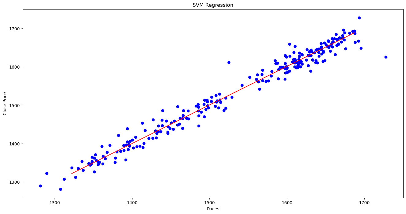
↪ 7. Predicting Close Price with generated input data

Create input data in the x_test range in the interval of 1, and predict the Close Price for each generated input data.

      x_grid = np.arange(x_test.values.min(), x_test.values.max())
      # Reshape the data into a len(x_grid)*1 array, i.e. to make a column out of the x_grid values 
      x_grid = x_grid.reshape((len(x_grid), 1)) 
      #
      plt.figure(figsize=(16,8))
      plt.title('SVM Regression')
      plt.xlabel('Prices')
      plt.ylabel('Close Price')
      print("x", x.size)
      print("y", y.size)
      plt.scatter(x, y, color = "blue")
      plt.plot(x_grid, svr.predict(x_grid), color = 'red')
      plt.show()

Support Vector Regression (SVR)

↪ 9. Strengths and Weaknesses

Support Vector Regression (SVR), a powerful technique for regression tasks, offers several advantages but also comes with certain limitations. Strengths

SVR performs well even when the number of features (dimensions) is large. The kernel function maps the data into a higher-dimensional space where linear separation or fitting is easier.

The choice of the kernel (linear, polynomial, radial basis function (RBF), sigmoid, etc.) allows SVR to model various types of relationships between the independent and the dependent variable. This flexibility makes it adaptable to different datasets.

Compared to other algorithms like neural networks, SVR is relatively memory efficient, especially with the use of efficient kernel implementations.

The epsilon-insensitive loss function used in SVR makes it less sensitive to outliers than methods that penalize all prediction errors equally.

Weaknesses

Training an SVR model can be computationally expensive, especially with large datasets. The computational complexity is related to the size of the training set and the choice of kernel.

SVR has several hyperparameters (like C, epsilon, and kernel parameters) that significantly influence its performance. Finding optimal hyperparameter values often requires experimentation and techniques like cross-validation or grid search, which can be time-consuming.