Logistic Regression

Logistic regression is a statistical method used for binary classification, meaning it predicts the probability of an event belonging to one of two categories. Unlike linear regression which predicts a continuous value, logistic regression models the probability of an outcome using a logistic (sigmoid) function, which squashes the output between 0 and 1. This makes it suitable for problems where the dependent variable is categorical with two possible outcomes (e.g.,UP or DOWN).

Logistic regression fits an S-shaped curve to the data, and a linear combination of the independent variables determine the position of this curve.

This module outlines the following steps:

➤ 1. Import data

➤ 2. Prepare data

➤ 3. Split data

➤ 4. Model training

➤ 5. Prediction

➤ 6. Confusion Matrix

➤ 7. Classification Report

➤ 8. Model Coefficients

➤ 9. Visualize the Model Coefficients

➤ 10. Strengths and Weaknesses

Logistic Regression

↪ 1. Import data

Import data using read_csv() function.

      import pandas as pd
      import numpy as np
      data = pd.read_csv('https://raw.githubusercontent.com/csxplore/data/main/andromeda-technical.csv', 
                       header=0)
      print(data.columns)

      ---Output---
      # Index(['Symbol', 'Series', 'Date', 'Prev Close', 'Open Price', 'High Price',
      #       'Low Price', 'Last Price', 'Close Price', 'Average Price',
      #       'Total Traded Quantity', 'Turnover', 'No. of Trades', 'Deliverable Qty',
      #       '% Dly Qt to Traded Qty', 'SMA20', 'SMA50', 'diff', 'UP'],
      #      dtype='object')

Logistic Regression

↪ 2. Prepare data

      print(data.shape)

      ---Output---
      # (250, 19)

Choose the required columns for analysis. This exercise predicts the Close Price using the Previous Close Price.

      data = data.dropna()
      data['UP2'] = np.where(data['UP'] == 'UP', 1, 0)
      data2 = data[['Open Price','Prev Close','SMA20','UP2']]
      print(data2.head(5))

      ---Output---
      #     Open Price  Prev Close      SMA20  UP2
      # 49     1428.00     1427.05  1394.8775    1
      # 50     1461.35     1462.05  1397.6725    1
      # 51     1486.50     1466.30  1401.3975    1
      # 52     1485.00     1485.70  1407.7900    0
      # 53     1494.80     1485.15  1414.4950    1
 
      X = data[['Open Price','Prev Close','SMA20']]
      y = data[['UP2']]

Logistic Regression

↪ 3. Split data

Split the data into training and test sets.

      from sklearn.model_selection import train_test_split
      X_train, X_test, y_train, y_test = train_test_split(X, y, test_size=0.2, random_state=42)

The code above performs a train-test split on a dataset. It utilizes the train_test_split() function to divide the data into training and testing sets. X represents the input features or independent variables, and y represents the corresponding target or dependent variable. The split is performed such that 20% of the data is allocated to the test set (test_size=0.2), while the remaining 80% is used for training. The random_state=42 argument ensures that the split is reproducible.

Logistic Regression

↪ 4. Model training

The code below demonstrates the core steps of training and using a logistic regression model with scikit-learn. First, it initializes a LogisticRegression model object, specifying solver='liblinear' for the optimization algorithm (suitable for smaller datasets) and setting random_state=42 for reproducibility of results. The model.fit(X_train, y_train) then trains the model using the provided training data, X_train (the features) and y_train (the corresponding binary target variable). During training, the model learns the optimal coefficients that best predict the probability of each class based on the provided features.

      from sklearn.linear_model import LogisticRegression
      lr = LogisticRegression(solver='liblinear', random_state=42) 
      lr.fit(X_train, y_train)

Logistic Regression

↪ 5. Prediction

The code below uses the trained logistic regression model to make predictions on new, unseen data.

      prediction = lr.predict(X_test)

The code compares the model's predictions to the actual values from the test dataset (y_test). It creates a Pandas DataFrame to display the first 5 'Actual' versus 'Predicted' values, providing a quick visual check of the model's performance on unseen data.

      y_pred = pd.DataFrame(prediction, columns=['Pred'])
      dframe = pd.concat([y_test.reset_index(drop=True).astype(float),y_pred], axis=1)
      dframe.columns = ['Actual', 'Predicted']
      graph = dframe.head(5)
      print(graph)

      ---Output---
      #      Actual  Predicted
      # 0     1.0          1
      # 1     0.0          0
      # 2     0.0          0
      # 3     1.0          1
      # 4     1.0          1

The code below demonstrates how to use a trained logistic regression model to predict an outcome for a new, unseen data point.

      input = [[1461.35,  1462.05,  1397.6725]]
      Predict_Close_Price= lr.predict(input)
      print("Predicted Value: ", Predict_Close_Price)

      ---Output---
      # Predicted Value:  [1]

Logistic Regression

↪ 6. Confusion Matrix

The code below calculates and displays a confusion matrix to evaluate the performance of a classification model. It uses the confusion_matrix function to generate a confusion matrix, which summarizes the model's predictions against the true labels.

From this matrix, the code extracts the individual counts for True Positives (TP), False Positives (FP), True Negatives (TN), and False Negatives (FN).

      from sklearn.metrics import confusion_matrix
      cm = confusion_matrix(y_test, prediction)
      print(cm)

      ---Output---
      # [[11  7]
      #  [ 3 20]]

The .ravel() method flattens the confusion matrix into a 1D array. A typical 2×2 confusion matrix (for binary classification) looks like this: [[TN, FP], [FN, TP]]

      TN, FP, FN, TP = confusion_matrix(y_test, prediction).ravel()
      print('True Positive (TP)  = ', TP)
      print('False Positive (FP) = ', FP)
      print('True Negative (TN)  = ', TN)
      print('False Negative (FN) = ', FN)

      ---Output---
      # True Positive (TP)  =  20
      # False Positive (FP) =  7
      # True Negative (TN)  =  11
      # False Negative (FN) =  6

Accuracy score can be calculated using the following formula.

      accuracy =  (TP+TN) / (TP+FP+TN+FN)
      print('Accuracy of the classification = {:0.3f}'.format(accuracy))

      ---Output---
      # Accuracy of the classification = 0.756

Alternatively, the accuracy_score() function calculates the accuracy of a classification model's predictions.

      from sklearn.metrics import accuracy_score
      accuracy = accuracy_score(y_test, prediction)
      print(f"Accuracy: {accuracy}")

      ---Output---
      # Accuracy:0.7560975609756098

Logistic Regression

↪ 7. Classification Report

The classification_report() function generates a text report showing the main classification metrics for each class in the dataset.

      from sklearn.metrics import classification_report
      print(classification_report(y_test, prediction))

      ---Output---
      #                precision    recall  f1-score   support
      #
      #             0       0.79      0.61      0.69        18
      #             1       0.74      0.87      0.80        23
      #
      #      accuracy                           0.76        41
      #     macro avg       0.76      0.74      0.74        41
      #  weighted avg       0.76      0.76      0.75        41

precision: The ratio of true positives to the total predicted positives (true positives + false positives). It measures how many of the positively predicted instances were actually positive.

recall (Sensitivity): The ratio of true positives to the total actual positives (true positives + false negatives). It measures how many of the actual positive instances were correctly predicted.

f1-score: The harmonic mean of precision and recall. It provides a balanced measure that considers both precision and recall. A higher f1-score indicates better performance.

support: The number of actual instances in each class in the test set.

Logistic Regression

↪ 8. Model Coefficients

The code below focuses on extracting and visualizing the coefficients of a trained logistic regression model. It extracts the coefficients learned by the trained model using lr.coef_[0]. These coefficients are then organized into a Pandas DataFrame coef_df, where each row contains a feature name and its corresponding coefficient. An additional column, 'abs_coefficient', is calculated, which represents the absolute value of the coefficient. The DataFrame is then sorted in descending order to reveal the features with the largest influence on the model.

      feature_names = ['Open Price','Prev Close','SMA20']
      coefs = lr.coef_[0]
      coef_df = pd.DataFrame({'feature': feature_names, 'coefficient': coefs})
      coef_df['abs_coefficient'] = abs(coef_df['coefficient'])
      coef_df = coef_df.sort_values('abs_coefficient', ascending = False)
      print(coef_df)

      ---Output---
      #        feature  coefficient  abs_coefficient
      #  0  Open Price     0.078564         0.078564
      #  1  Prev Close    -0.075680         0.075680
      #  2       SMA20    -0.002791         0.002791

Logistic Regression

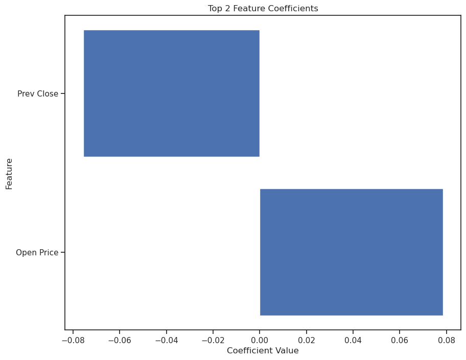
↪ 9. Visualize the Model Coefficients

Finally, the code generates a horizontal bar chart to visualize the coefficients of the two most influential features. It uses matplotlib to create a bar chart of the top two features from the sorted coef_df against their raw coefficient values. This visualization helps in quickly identifying which features are most impactful in determining the outcome predicted by the logistic regression model, as well as whether the influence is positive or negative.

      plt.figure(figsize=(10, 8))
      plt.barh(coef_df['feature'][:2], coef_df['coefficient'][:2])
      plt.xlabel("Coefficient Value")
      plt.ylabel("Feature")
      plt.title("Top 2 Feature Coefficients")
      plt.savefig(svgpath + "logreg1.png",  bbox_inches='tight')
      plt.show()

Logistic Regression

↪ 10. Strengths and Weaknesses

Strengths

Relatively easy to understand and implement, even for those without advanced statistical backgrounds.

Computationally inexpensive and can be trained relatively quickly, even on moderately sized datasets.

Efficient memory usage, making it suitable for environments with limited resources.

Provides probabilities for class membership, not just binary predictions. This allows for more nuanced decision-making and threshold adjustment.

Built on solid statistical theory, allowing for statistical inference (confidence intervals, p-values) and model validation.

Effective for a wide range of binary classification problems across various domains.

Weaknesses

Assumes a linear relationship between the independent and the dependent variables. If this assumption is violated, the model's performance suffers significantly.

Primarily designed for binary classification and its extensions for multiclass classification. It is not a suitable model for regression tasks or problems with more complex outcome variables.

Outliers can have a significant impact on the model.

A High correlation between independent variables can lead to unstable coefficient estimates and inflated variance, making interpretation difficult.