KNN Regression

K-Nearest Neighbors (KNN) regression is a non-parametric method used for predicting continuous values. Unlike linear regression, it doesn't assume a specific functional form for the relationship between the independent and the dependent variables. Instead, it operates based on the principle that similar data points tend to have similar outcomes. When a prediction is needed for a new data point, KNN regression identifies the 'k' closest data points (neighbors) from the training set, based on a chosen distance metric (like Euclidean or Manhattan distance) in the feature space. The prediction is then determined by averaging the outcome values of these 'k' nearest neighbors.

  ➤ 1. Import data

  ➤ 2. Prepare data

  ➤ 3. Split data

  ➤ 4. Model training

  ➤ 5. Prediction

  ➤ 6. Actual vs. Predicted Graph

  ➤ 7. Evaluate the model

  ➤ 8. Strengths and Weaknesses

KNN Regression

↪ 1. Import data

Import data using read_csv() function.

      import pandas as pd
      import numpy as np
      data = pd.read_csv('https://raw.githubusercontent.com/csxplore/data/main/andromeda-technical.csv', 
                       header=0)
      print(data.columns)

      ---Output---
      # Index(['Symbol', 'Series', 'Date', 'Prev Close', 'Open Price', 'High Price',
      #       'Low Price', 'Last Price', 'Close Price', 'Average Price',
      #       'Total Traded Quantity', 'Turnover', 'No. of Trades', 'Deliverable Qty',
      #       '% Dly Qt to Traded Qty', 'SMA20', 'SMA50', 'diff', 'UP'],
      #      dtype='object')

KNN Regression

↪ 2. Prepare data

      print(data.shape)

      ---Output---
      # (250, 19)

Choose the required columns for analysis. This exercise predicts the Close Price using the Previous Close Price.

      data2 = data.dropna()
      data2 = data[['Prev Close', 'Close Price']]
      print(data2.head(5))

      ---Output---
      #    Prev Close  Close Price
      # 0     1401.55      1388.95
      # 1     1388.95      1394.85
      # 2     1394.85      1385.10
      # 3     1385.10      1380.30
      # 4     1380.30      1378.45
 
      X = data[['Prev Close']]
      y = data['Close Price']

KNN Regression

↪ 3. Split data

Split the data into training and test sets.

      from sklearn.model_selection import train_test_split
      X_train, X_test, y_train, y_test = train_test_split(X, y, test_size=0.2, random_state=42)

The code above performs a train-test split on a dataset. It utilizes the train_test_split() function to divide the data into training and testing sets. X represents the input features or independent variables, and y represents the corresponding target or dependent variable. The split is performed such that 20% of the data is allocated to the test set (test_size=0.2), while the remaining 80% is used for training. The random_state=42 argument ensures that the split is reproducible.

KNN Regression

↪ 4. Model training

Standardize the features This step is generally recommended for KNN methods since distance computation will be significantly impacted by feature scaling. The code below standardizes the training and testing feature data using StandardScaler() function. It first initializes the scaler and then uses fit_transform() function on the training data (X_train) to calculate the mean and standard deviation of each feature, and then transform it to have zero mean and unit standard deviation.

The scaler then applies the same transformation using transform() on the test data (X_test), ensuring consistent scaling across both datasets based on the training data's statistics. This preprocessing step is crucial for many machine learning algorithms, including KNN, as it prevents features with larger scales from dominating the distance calculations.

      from sklearn.preprocessing import StandardScaler
      scaler = StandardScaler()
      X_train_scaled = scaler.fit_transform(X_train)
      X_test_scaled = scaler.transform(X_test)

The code below initializes and trains a K-Nearest Neighbors (KNN) regressor model. It first imports the KNeighborsRegressor class. Then, it creates an instance of the regressor, setting the number of neighbors (k) to 5. Finally, the fit method is used to train the model using the scaled training features (X_train_scaled) and corresponding training target values (y_train).

      from sklearn.neighbors import KNeighborsRegressor
      knn_regressor = KNeighborsRegressor(n_neighbors=5)
      knn_regressor.fit(X_train_scaled, y_train)

KNN Regression

↪ 5. Prediction

The code below uses the trained K-Nearest Neighbors (KNN) regression model to make predictions on new, unseen data.

      prediction = knn_regressor.predict(X_test_scaled)

The code compares the model's predictions to the actual values from the test dataset (y_test). It creates a Pandas DataFrame to display the first 5 'Actual' versus 'Predicted' values, providing a quick visual check of the model's performance on unseen data.

      y_pred = pd.DataFrame(prediction, columns=['Pred'])
      dframe = pd.concat([y_test.reset_index(drop=True).astype(float),y_pred], axis=1)
      dframe.columns = ['Actual', 'Predicted']
      graph = dframe.head(5)
      print(graph)

      ---Output---
      #     Actual  Predicted
      # 0  1597.65    1621.98
      # 1  1367.40    1356.59
      # 2  1458.65    1451.79
      # 3  1464.85    1469.85
      # 4  1611.15    1505.07

The code below demonstrates how to use a trained KNN regression model to predict an outcome for a new, unseen data point. First, the new input value 1508.80 is scaled using the previously fitted StandardScaler object, ensuring it is processed using the same scaling parameters applied to the training data. Then, the scaled input is passed to the predict() function of the trained KNN regressor, which calculates and returns the predicted outcome value.

      scaled_input = scaler.transform([[1508.80]])
      Predict_Close_Price= knn_regressor.predict(scaled_input)
      print("Predicted Value: ", Predict_Close_Price)

      ---Output---
      # Predicted Value: [1510.36]

KNN Regression

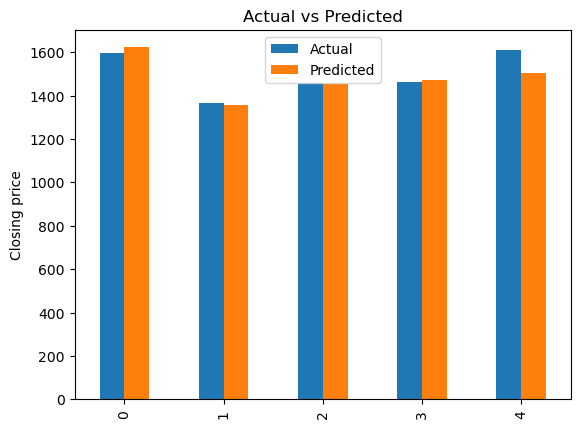
↪ 6. Actual vs. Predicted Graph

The code below generates a bar chart that compares actual and predicted values. It uses the matplotlib.pyplot library to create a bar plot from the DataFrame “graph”.

      import matplotlib.pyplot as plt
      graph.plot(kind='bar')
      plt.title('Actual vs Predicted')
      plt.ylabel('Closing price')
      plt.show()

KNN Regression

↪ 7. Evaluate the model

This code evaluates the performance of a regression model using two key metrics: Mean Squared Error (MSE) and R-squared (R²). The mean_squared_error function computes the average squared difference between the model's predictions (y_pred) and the true values (y_test). A lower MSE indicates better accuracy.

      from sklearn.metrics import mean_squared_error
      mse = mean_squared_error(y_test, y_pred)
      print(f"Mean Squared Error: {mse}")

      ---Output---
      # Mean Squared Error: 527.0895719999993

The MSE, which is 527, represents the average squared difference between the model's predictions and the actual values in the test set. A lower MSE is better, indicating that the model's predictions are, on average, close to the true values.

The r2_score function calculates the R-squared, a measure of how well the model fits the data, ranging from 0 to 1. A higher R² (closer to 1) suggests a better fit, indicating that the model explains a larger proportion of the variance in the dependent variable.

      from sklearn.metrics import  r2_score
      r2 = r2_score(y_test, y_pred)
      print(f"R-squared: {r2}")

      ---Output---
      # R-squared: 0.9626016860080269

The R-squared value of 0.97 indicates that the model explains approximately 97% of the variance in the data. This is a high R-squared, suggesting a good model fit to the test data.

KNN Regression

↪ 8. Strengths and Weaknesses

Strengths

Weaknesses