K-means Clustering

K-Means clustering is an unsupervised machine learning algorithm used to partition a dataset into a predefined number of clusters (k). The algorithm aims to group data points in such a way that the within-cluster sum of squares (WCSS), also known as inertia, is minimized. The core idea of K-Means involves iteratively assigning each data point to the nearest cluster center (centroid) and then recomputing the centroids based on the newly assigned cluster members. This iterative process continues until the cluster assignments no longer change or a predefined number of iterations is reached.

This module outlines the following steps:

  ➤ 1. Import data

  ➤ 2. Analyze data

  ➤ 3. Determine the optimal number of clusters

  ➤ 4. Model training

  ➤ 5. Get Cluster Labels and Centers

  ➤ 6. Visualize the clusters

  ➤ 7. Accuracy Score

  ➤ 8. Confusion Matrix

  ➤ 9. Silhouette score

  ➤ 10. Strengths and Weaknesses

K-means Clustering

↪ 1. Import data

The “Breast Cancer” dataset, a toy binary classification dataset included in the scikit-learn library, serves as a popular example for demonstrating machine learning clustering tasks. The dataset's features are calculated from digitized images of fine needle aspirates (FNA) of breast masses and are used to predict if a mass is malignant (cancerous) or benign (non-cancerous).

The sklearn.datasets package provides access to the “Breast Cancer” dataset, which is loaded using the load_breast_cancer() function. The returned dataset object is stored in the variable bc. This object contains the features, targets (labels), and descriptive metadata. Specifically, bc.feature_names holds a list of the names of all 30 features (for example, “mean radius” and “texture”).

      # Load Breast Cancer dataset
      from sklearn.datasets import load_breast_cancer
      bc = load_breast_cancer()
 
      # Access the data and target attributes
      print(bc.feature_names)

      ---Output---
      # ['mean radius' 'mean texture' 'mean perimeter' 'mean area'
      #  'mean smoothness' 'mean compactness' 'mean concavity'
      #  'mean concave points' 'mean symmetry' 'mean fractal dimension'
      #  'radius error' 'texture error' 'perimeter error' 'area error'
      #  'smoothness error' 'compactness error' 'concavity error'
      #  'concave points error' 'symmetry error' 'fractal dimension error'
      #  'worst radius' 'worst texture' 'worst perimeter' 'worst area'
      #  'worst smoothness' 'worst compactness' 'worst concavity'
      #  'worst concave points' 'worst symmetry' 'worst fractal dimension']

The dataset contains a total of 569 instances (or data points).

      data = bc.data
      print("Number of Instances, Number of features", data.shape)

      ---Output---
      # Number of Instances, Number of features (569, 30)

The bc.target_names attribute provides the labels for the classifications. It has two classes:
      Malignant (0): Indicates a cancerous breast mass.
      Benign (1): Indicates a non-cancerous breast mass.
 

      print(bc.target_names)
      target = bc.target

      ---Output---
      # ['malignant' 'benign']

K-means Clustering

↪ 2. Analyze data

The code below uses the load_breast_cancer() function with the return_X_y=True argument to separate the features (data) and target variable (labels) and the as_frame = True to load data into a pandas DataFrame. The feature data is assigned to the variable df, and the target variable is assigned to m.

      df, m = load_breast_cancer(return_X_y=True, as_frame = True)
      print("Number of Instances", df.shape)

      ---Output---
      # Number of Instances (569, 30)

Next, the code explores the target variable m. It uses the .value_counts() method to display the number of occurrences of each unique value within the target variable. The printed output indicates the number of instances in the 'malignant' category and the number in the 'benign' category, revealing the class distribution in the dataset.

      print("m values", m.value_counts()) # 0 = malignant, 1 = benign

      ---Output---
      # m values target
      # 1    357
      # 0    212

K-means Clustering

↪ 3. Determine the optimal number of clusters

The code below implements the Elbow Method to determine the optimal number of clusters for a K-Means clustering algorithm. It starts by importing matplotlib.pyplot for plotting and KMeans from sklearn.cluster for clustering. An empty list 'wccs' is initialized to store the within-cluster sum of squares (WCSS) values, also known as inertia. The code then iterates through a range of cluster numbers from 1 to 30. In each iteration, it initializes a KMeans object with the current number of clusters (i), using k-means++ for initialization, max_iter=300 for the maximum iterations, n_init=10 for the number of initializations, and a random_state for reproducibility. The K-Means model is then trained on the data X, and the inertia (WCSS) is appended to the 'wccs' list.

Finally, the code plots the inertia values against the corresponding number of clusters using matplotlib. The resulting plot, called the “Elbow Method” plot, is a line graph where the x-axis represents the number of clusters and the y-axis represents the within-cluster sum of squares. The “elbow” point, which represents a point where the rate of decrease in inertia starts to slow down, helps visually determine a suitable number of clusters for the data.

      import matplotlib.pyplot as plt
      from sklearn.cluster import KMeans
      wccs = []
      for i in range(1, 30):
          kmeans = KMeans(n_clusters = i, init = 'k-means++', max_iter = 300, n_init = 10, random_state = 0)
          kmeans.fit(X)
          wccs.append(kmeans.inertia_)
      plt.plot(range(1, 30), wccs)
      plt.title('The Elbow Method')
      plt.xlabel('Number of clusters')
      plt.ylabel('Inertia')
      plt.show()

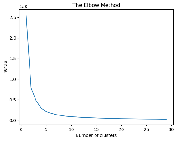
Based on the plot above, an elbow point is observed at two clusters, where the rate of decrease in the WCSS begins to slow. This is consistent with the two classes in the Breast Cancer dataset.

K-means Clustering

↪ 4. Model training

The code below prepares data and applies the K-Means clustering algorithm to the Breast Cancer dataset.

It extracts the feature data (bc.data) and target variable (bc.target) from a previously loaded dataset, assigning them to X and y, respectively. Then, it imports StandardScaler from scikit-learn for feature scaling, which is essential for distance-based algorithms like K-Means. A StandardScaler object is initialized, which is used for scaling the feature data by transforming X into X_scaled. Feature scaling standardizes the data that ensures each feature has a mean of 0 and a standard deviation of 1, which prevents features with larger values from dominating the clustering process.

      X = bc.data  # Features
      y = bc.target  # Target variable
 
      # Standardize the features
      from sklearn.preprocessing import StandardScaler
      scaler = StandardScaler()
      X_scaled = scaler.fit_transform(X)

Following data preparation, a KMeans clustering model is initialized with n_clusters=2 and a fixed random_state for reproducibility. The fit() method is then called on the kmeans object, using the scaled feature data (X_scaled). This step performs the clustering algorithm to group similar instances of the dataset into the specified number of clusters.

      kmeans = KMeans(n_clusters=2, random_state=42)
      kmeans.fit(X_scaled)

K-means Clustering

↪ 5. Get Cluster Labels and Centers

The code below extracts the cluster centers from the trained K-Means model using kmeans.cluster_centers_ and the predicted cluster labels for each data point using kmeans.labels_, storing them in cluster_centers and labels respectively.

      # Get cluster centers and labels
      cluster_centers = kmeans.cluster_centers_
      labels = kmeans.labels_

The code below combines the true class labels and the predicted cluster labels into a single, viewable pandas DataFrame for easier comparison. It converts the cluster labels (labels) from the previous K-Means clustering process into a pandas DataFrame named 'clusterdf'. Similarly, it converts the true class labels (y) into another pandas DataFrame named 'ydf'. Using the pd.concat() function, it combines 'ydf' and 'clusterdf' into a single DataFrame named 'dframe', concatenating them column-wise (specified by axis=1). The code prints the first five rows of the dframe for a side-by-side comparison.

      import pandas as pd
      clusterdf = pd.DataFrame(labels)
      ydf = pd.DataFrame(y)
      dframe = pd.concat([ydf,clusterdf], axis=1)
      dframe.columns = ['True Label y','Predicted']
      print(dframe.head(5))

      ---Output---
      #     True Label y  Predicted
      #  0             0          0
      #  1             0          0
      #  2             0          0
      #  3             0          0
      #  4             0          0

K-means Clustering

↪ 6. Visualize the clusters

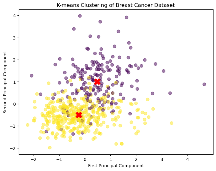
The code below generates a visualization of the K-Means clustering results using matplotlib. It generates a scatter plot where the x-axis and y-axis represent the second and third scaled features of the data, respectively (using X_scaled[:, 1] and X_scaled[:, 2]). The parameter c=labels sets the color of each point according to the cluster assignment stored in labels, and cmap='viridis' sets the colormap for visualization. Also, the size of each data point is set to 50 and the alpha to 0.5 to improve visualization.

Next, the code adds the cluster centers to the scatter plot. The cluster centers are represented by large red crosses (using the marker='X' parameter), making them easily distinguishable from the data points. Similar to the data points, the x and y coordinates for the cluster centers are also taken from the second and third columns from cluster_centers.

      # Visualize the clusters (using only the first two components for simplicity)
      plt.figure(figsize=(8, 6))
      plt.scatter(X_scaled[:, 1], X_scaled[:, 2], c=labels, cmap='viridis', s=50, alpha=0.5)
      plt.scatter(cluster_centers[:, 1], cluster_centers[:, 2], c='red', s=200, marker='X')
      plt.xlabel('First Component')
      plt.ylabel('Second Component')
      plt.title('K-means Clustering of Breast Cancer Dataset')
      plt.show()

K-means Clustering

↪ 7. Accuracy Score

The code below calculates the number of data points that were correctly assigned to the “correct” clusters by comparing the predicted cluster labels (labels) with the true class labels (y). This is done by summing the boolean results of (y == labels). The result of this sum, representing the number of correctly labeled data points, is stored in correct_labels.

      correct_labels = sum(y == labels)
      print("Result: %d out of %d samples were correctly labeled." % (correct_labels, y.size))
      print('Accuracy score: {0:0.2f}'. format(correct_labels/float(y.size)))

      ---Output---
      # Result: 518 out of 569 samples were correctly labeled.
      # Accuracy score: 0.91

Alternatively, the accuracy_score() function calculates the accuracy of a classification model's predictions.

      from sklearn.metrics import accuracy_score
      accuracy = accuracy_score(ydf, clusterdf)
      print(f"Accuracy: {accuracy}")

      ---Output---
      # Accuracy: 0.9103690685413005

K-means Clustering

↪ 8. Confusion Matrix

The code below calculates and displays a confusion matrix to evaluate the performance of a classification model. It uses the confusion_matrix() function to generate a confusion matrix, which summarizes the model's predictions against the true labels.

From this matrix, the code extracts the individual counts for True Positives (TP), False Positives (FP), True Negatives (TN), and False Negatives (FN).

      from sklearn.metrics import confusion_matrix
      cm = confusion_matrix(ydf, clusterdf)
      print(cm)

      ---Output---
      # [[175  37]
      #  [ 14 343]

The .ravel() method flattens the confusion matrix into a 1D array. A typical 2×2 confusion matrix (for binary classification) looks like this: [[TN, FP], [FN, TP]]

      TN, FP, FN, TP = confusion_matrix(ydf, clusterdf).ravel()
      print('True Positive (TP)  = ', TP)
      print('False Positive (FP) = ', FP)
      print('True Negative (TN)  = ', TN)
      print('False Negative (FN) = ', FN)

      ---Output---
      # True Positive (TP)  =  343
      # False Positive (FP) =  37
      # True Negative (TN)  =  175
      # False Negative (FN) =  14

Accuracy score can be calculated using the following formula.

      accuracy =  (TP+TN) / (TP+FP+TN+FN)
      print('Accuracy of the classification = {:0.3f}'.format(accuracy))

      ---Output---
      # Accuracy of the classification = 0.910

K-means Clustering

↪ 9. Silhouette score

The code below calculates and displays the silhouette score, a metric used to evaluate the quality of clustering results. First, it imports the silhouette_score() function from sklearn.metrics, which is used to compute the silhouette coefficient for each data point. The function takes the scaled feature data (X_scaled) and the cluster labels (labels) as input. The average silhouette score, calculated from these individual silhouette coefficients, is stored in the variable silhouette_avg. This score provides a measure of how similar an object is to its own cluster compared to other clusters; it ranges from -1 to 1, with higher scores indicating better-defined clusters.

      from sklearn.metrics import silhouette_score
      silhouette_avg = silhouette_score(X_scaled, labels)
      print(f"Average Silhouette Score: {silhouette_avg:.2f}")

      ---Output---
      # Average Silhouette Score: 0.34

The average silhouette score of 0.34 indicates that the data points are not very well separated with these clusters, as scores closer to 1 are desirable.

K-means Clustering

↪ 10. Strengths and Weaknesses

Strengths

Weaknesses