Fit the model using the sklearn LinearRegression
This module covers the following steps:
➤ 1. Import Data
➤ 2. Coefficient of determination
➤ 3. Predict and Test the model
➤ 4. Compare the actual and predicted values
➤ 5. Actual vs. Predicted Graph
➤ 6. Metrics
➤ 7. Predicting Close Price
➤ 8. Strengths and Weaknesses
Fit the model using the sklearn LinearRegression
↪ 1. Import Data
Import the pre-processed data for analysis. Subsequently, the data will be partitioned into training and test sets to facilitate the analysis.
      # Import required libraries.
      import pandas as pd                                 # Matplotlib is the fundamental plotting library
      import matplotlib.pyplot as plt                     # Seaborn builds upon Matplotlib, offering a
      import seaborn as sns                               # higher-level interface for statistical visualization.
      import numpy as np

      # Set default style and color scheme for Seaborn plots.
      sns.set(style="ticks", color_codes=True)

      # Import data
      data = pd.read_csv('https://raw.githubusercontent.com/csxplore/data/main/andromeda-cleaned.csv',
                       header=0)
      data = data[['Prev Close','Close Price']]
      x=data[['Prev Close']]
      y=data[['Close Price']]

      # Split the data into training and test sets.
      from sklearn.model_selection import train_test_split
      x_train, x_test, y_train, y_test = train_test_split(x,y, test_size=0.2,random_state=0)
Fit the model using the sklearn LinearRegression
↪ 2. Coefficient of determination
The coefficient of determination, commonly known as R-squared (R²), is a statistical measure used in linear regression. It quantifies the proportion of variance in the dependent variable (y) that is predictable from the independent variable (x), indicating the model's goodness of fit.
      from sklearn.linear_model import LinearRegression   #for linear regression model
      lm=LinearRegression()
      lm.fit(x_train,y_train)

      print("Slope: ", lm.coef_)
      print("Intercept: ", lm.intercept_)

      ---Output---
      # Slope:  [[0.99074645]]
      # Intercept:  [16.58736543]
The score() method returns the model's coefficient of determination.
      print('Coefficient of determination: ',lm.score(x_train,y_train))

      ---Output---
      # Coefficient of determination:  0.9766415429151323
The model explains 97.66% of the variance in the dependent variable 'Close Price', indicating
a strong relationship between 'Prev Close' and 'Close Price'.
Fit the model using the sklearn LinearRegression
↪ 3. Predict and Test the model
predictions = lm.predict(x_test)
The r2_score() method from sklearn.metrics calculates the coefficient of determination for predictions, measuring how well the model's predictions align with the actual values.
      from sklearn.metrics import r2_score
      print('Coefficient of determination: ', r2_score(y_test, predictions))

      ---Output---
      # Coefficient of determination:  0.9533174640966606
Fit the model using the sklearn LinearRegression
↪ 4. Compare the actual and predicted values
      y_pred = pd.DataFrame(predictions, columns=['Pred'])
      dframe = pd.concat([y_test.reset_index(drop=True).astype(float),y_pred], axis=1)
      dframe.columns = ['Actual','Predicted']
      graph = dframe.head(10)
      print(graph)

      ---Output---
      # -    Actual    Predicted
      # 0  1671.80  1665.338077
      # 1  1617.65  1626.698965
      # 2  1409.80  1404.276386
      # 3  1600.65  1601.187244
      # 4  1568.30  1599.304826
      # 5  1644.10  1638.736535
      # 6  1564.35  1570.622716
      # 7  1389.55  1417.354240
      # 8  1486.10  1442.667811
      # 9  1590.90  1570.375029
Fit the model using the sklearn LinearRegression
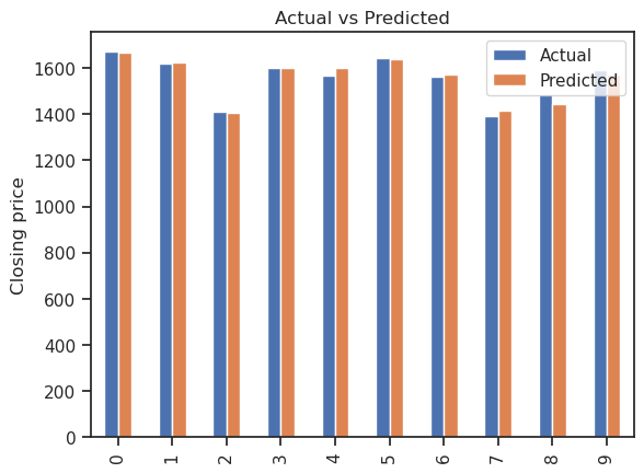
↪ 5. Actual vs. Predicted Graph
      graph.plot(kind='bar')
      plt.title('Actual vs Predicted')
      plt.ylabel('Closing price')
      plt.show()

Fit the model using the sklearn LinearRegression
↪ 6. Metrics
The model's precision depends on the problem type that needs to be solved. Typically, use
Mean Absolute Error (MAE) Mean Absolute Error (MAE) is the mean of the absolute value of the difference between the predicted value and the actual value. The MAE tells how big of an error in the predicted value is expected in the model.
Mean squared error (MSE) Mean squared error (MSE) or Mean Squared Deviation (MSD)is the average squared distance between the actual and predicted values. The MSE represents the average squared residual.
Squaring the differences eliminates negative values of the differences and ensures that the MSE is positive. However, squaring increases the impact of larger errors, and these calculations disproportionately penalize larger errors more than smaller errors.
Variance is the average squared deviation of the observations from the mean. The MSE in contrast is the average of squared deviations of the predictions from the actual values (residuals).
The Root Mean Square Error (RMSE) The Root Mean Square Error (RMSE) measures the average difference between the actual and predicted values. The RMSE is the standard deviation of the residuals. Residuals represent the distance between the regression line and the data points.
Fit the model using the sklearn LinearRegression
↪ 6. Metrics
      from sklearn import metrics
      import math

      print('Mean Absolute Error:     ', metrics.mean_absolute_error(y_test.astype(float),y_pred))
      print('Mean Squared Error:      ', metrics.mean_squared_error(y_test.astype(float),y_pred))
      print('Root Mean Squared Error: ', math.sqrt(metrics.mean_squared_error(y_test.astype(float),y_pred)))

      ---Output---
      # Mean Absolute Error:      15.329547985270242
      # Mean Squared Error:       496.08485332380906
      # Root Mean Squared Error:  22.272962383208235
Fit the model using the sklearn LinearRegression
↪ 7. Predicting Close Price
      Predict_Close_Price= lm.predict([[1508.80]])
      print("Predicted Value: ", Predict_Close_Price)

      ---Output---
      # Predicted Value:  [[1511.42561533]]
Fit the model using the sklearn LinearRegression
↪ 8. Strengths and Weaknesses
Strengths
Weakness
