
Decision Tree Regression
Decision tree regression, a versatile and interpretable technique for predicting continuous values, helps reveal the underlying relationships between independent and dependent variables. It trains a model in the form of a tree structure to make predictions about future data.
This module outlines the following steps:
➤ 1. Import data
➤ 2. Review data
➤ 3. Split data
➤ 4. Fit decision tree regressor
➤ 5. Compare actual and predicted values
➤ 6. Decision Tree
➤ 7. Predicting Close Price with Generated Input Data
➤ 8. Predict 20 days into the future
➤ 9. Strengths and Weaknesses
Decision Tree Regression
↪ 1. Import data
Import the pre-processed data for analysis. Subsequently, the data will be partitioned into training and test sets to facilitate the analysis.
      # Import required libraries.
      import pandas as pd                                 # Matplotlib is the fundamental plotting library
      import matplotlib.pyplot as plt                     # Seaborn builds upon Matplotlib, offering a
      import seaborn as sns                               # higher-level interface for statistical visualization.
      import numpy as np
Set default style and color scheme for Seaborn plots.
sns.set(style="ticks", color_codes=True)
Import data using read_csv() function.
      data = pd.read_csv('https://raw.githubusercontent.com/csxplore/data/main/andromeda-cleaned.csv',
                       header=0)
      print(data.columns)

      ---Output---
      # Index(['Symbol', 'Series', 'Date', 'Prev Close', 'Open Price', 'High Price',
      #        'Low Price', 'Last Price', 'Close Price', 'Average Price',
      #        'Total Traded Quantity', 'Turnover', 'No. of Trades', 'Deliverable Qty',
      #        '% Dly Qt to Traded Qty'],
      #       dtype='object')
The info() function can be used for checking the data type.
data.info()
---Output--- ## RangeIndex: 250 entries, 0 to 249 # Data columns (total 15 columns): # # Column Non-Null Count Dtype # --- ------ -------------- ----- # 0 Symbol 250 non-null object # 1 Series 250 non-null object # 2 Date 250 non-null object # 3 Prev Close 250 non-null float64 # 4 Open Price 250 non-null float64 # 5 High Price 250 non-null float64 # 6 Low Price 250 non-null float64 # 7 Last Price 250 non-null float64 # 8 Close Price 250 non-null float64 # 9 Average Price 250 non-null float64 # 10 Total Traded Quantity 250 non-null float64 # 11 Turnover 250 non-null float64 # 12 No. of Trades 250 non-null float64 # 13 Deliverable Qty 250 non-null float64 # 14 % Dly Qt to Traded Qty 250 non-null float64 # dtypes: float64(12), object(3) # memory usage: 29.4+ KB
Decision Tree Regression
↪ 2. Review data
The shape attribute display the data shape.
      print(data.shape)

      ---Output---
      # (250, 15)
Visualize the closing prices.
      plt.figure(figsize=(16,8))
      plt.title('Andromeda')
      plt.xlabel('Days')
      plt.ylabel('Close Price')
      plt.plot(data['Close Price'])
      plt.show()

Decision Tree Regression
↪ 3. Split data
Choose the required columns for analysis. This exercise predicts the Close Price using the Previous Close Price.
      data = data[['Prev Close','Close Price']]
      x=data[['Prev Close']]
      y=data[['Close Price']]
Split the data into training and test sets.
      from sklearn.model_selection import train_test_split
      x_train, x_test, y_train, y_test = train_test_split(x,y, test_size=0.2,random_state=0)
      print("x_train.shape: ", x_train.shape )
      print("x_test.shape: ", x_test.shape )
      print("y_train.shape: ", y_train.shape )
      print("y_test.shape", y_test.shape )

      ---Output---
      # x_train.shape:  (200, 1)
      # x_test.shape:  (50, 1)
      # y_train.shape:  (200, 1)
      # y_test.shape (50, 1)
Decision Tree Regression
↪ 4. Fit decision tree regressor
The DecisionTreeRegressor is the specific class representing a decision tree regression model.
      from sklearn.tree import DecisionTreeRegressor
      tree = DecisionTreeRegressor().fit(x_train, y_train)
The above code snippet imports the DecisionTreeRegressor() function to create a decision tree regression model. The second line creates an instance of the model, initializes it, and trains it using the provided training data (x_train and y_train). After this, the variable 'tree' holds a trained decision tree model, ready for making predictions on new, unseen data.
Predicting Close Price
      Predict_Close_Price= tree.predict(pd.DataFrame({'Prev Close': [1508.80]}))
      print("Predicted Value: ", Predict_Close_Price)

      ---Output---
      #Predicted Value:  [1508.35]
Decision Tree Regression
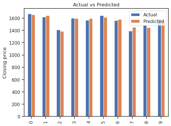
↪ 5. Compare actual and predicted values
      # tree_pred variable stores the predicted values output by the decision tree model.
      tree_pred = tree.predict(x_test)
      # y_pred variable holds the DataFrame containing the predictions.
      y_pred = pd.DataFrame(tree_pred, columns=['Pred'])
      # dframe variable holds the combined DataFrame
      dframe = pd.concat([y_test.reset_index(drop=True).astype(float),y_pred], axis=1)
      dframe.columns = ['Actual','Predicted']
      # dframe.head(10) selects the first 10 rows of the DataFrame and assigns them to the variable graph.
      graph = dframe.head(10)
      print(graph)

      ---Output---
      # - Actual  Predicted
      # 0  1446.15    1472.15
      # 1  1365.05    1353.75
      # 2  1587.80    1575.80
      # 3  1671.90    1658.45
      # 4  1673.10    1631.80
      # 5  1597.50    1599.15
      # 6  1627.30    1619.75
      # 7  1688.15    1670.30
      # 8  1647.30    1670.30
      # 9  1393.60    1391.80
Decision Tree Regression
↪ 5. Compare the actual and predicted values
      graph.plot(kind='bar')
      plt.title('Actual vs Predicted')
      plt.ylabel('Closing price')
      plt.show()
Decision Tree Regression
↪ 6. Decision Tree
DecisionTree algorithm splits the data set into 2 parts to minimize the mean squared error. The algorithm does this repetitively and forms a tree structure.
The plot_tree() function from the sklearn.tree module creates a graphical representation of a decision tree. The following code generates a visualization that focuses on how the 'Prev Close' variable contributes to predicting its target. The visualization shows the tree's structure up to a depth of two, with color-filled nodes.
      from sklearn.tree import plot_tree
      fig = plt.figure(figsize=(25,20))
      plot_tree(tree, feature_names =['Prev Close'],class_names =['Prev Close'],
                filled=True, max_depth=2 )
      plt.show()

Decision Tree Regression
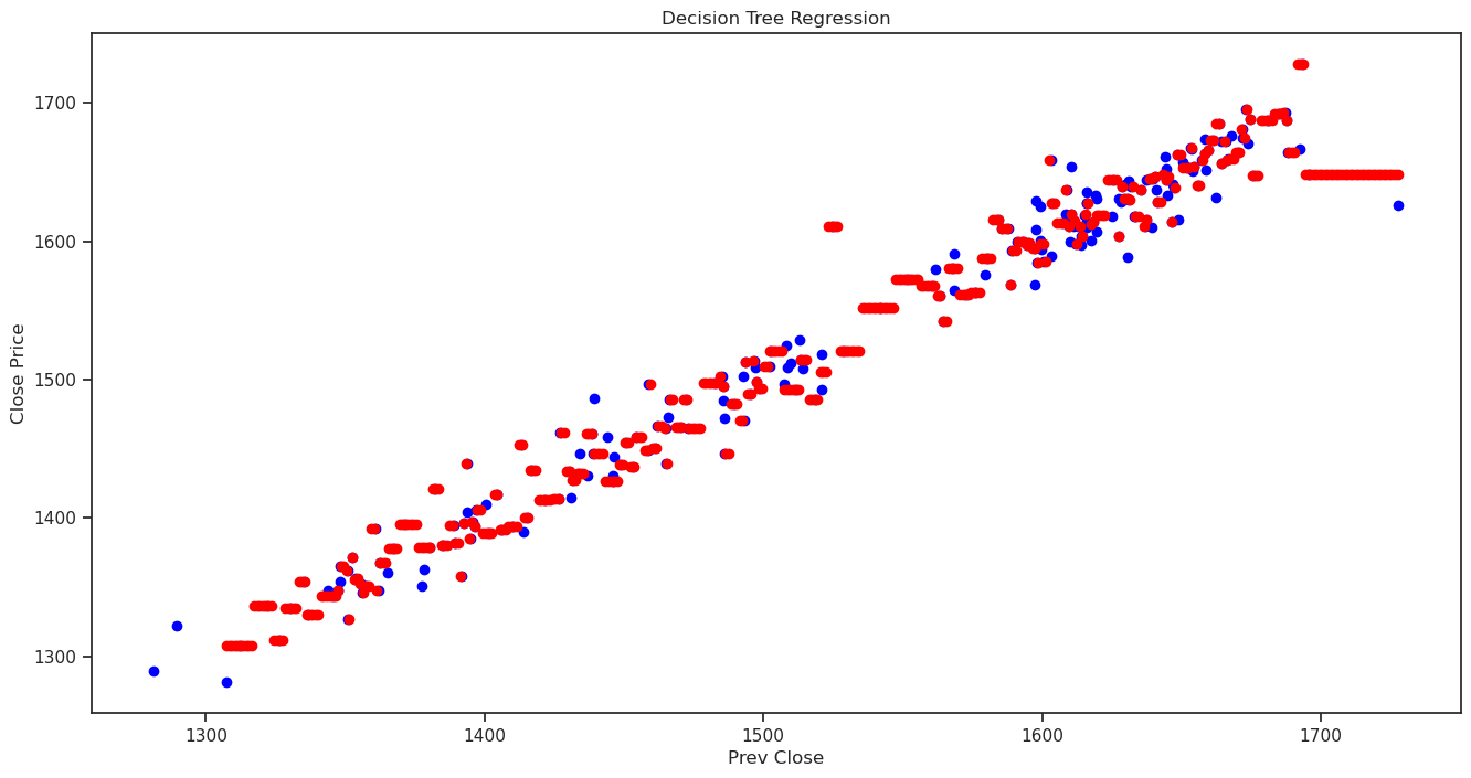
↪ 7. Predicting Close Price with generated input data
Create input data in the x_test range in the interval of 1, and predict the Close Price for each generated input data.
      X_grid = np.arange(x_test.values.min(), x_test.values.max())
      # Reshape the data into  a len(X_grid)*1 array, i.e. to make a column out of the X_grid values
      X_grid = X_grid.reshape((len(X_grid), 1))
      # Compare the predicted Close Price with the actual Close Price using scatter plot.
      plt.figure(figsize=(16,8))
      plt.title('Decision Tree Regression')
      plt.xlabel('Prev Close')
      plt.ylabel('Close Price')
      plt.scatter(x, y, color = "blue")
      plt.scatter(X_grid, tree.predict(X_grid), color = 'red')
      plt.show()
Decision Tree Regression
↪ 8. Predict 20 days into the future
      print(data.tail(5))

      ---Output---
      #     Prev Close  Close Price
      # 245     1615.80      1609.60
      # 246     1609.60      1615.80
      # 247     1615.80      1635.50
      # 248     1635.50      1636.75
      # 249     1636.75      1610.85
Last Close Price will be used to predict the Close Price for the next day.
      future_days = 20                  # Define the number of future dates for predicting
                                        # the Close Price
      pp = data['Close Price'].iloc[-1] # Last Close Price : [1610.85]

      i = 1
      while i < future_days:
         cp_pred = tree.predict(pd.DataFrame({'Prev Close': [pp.item()]}))
         new_row = pd.DataFrame({"Prev Close": [pp.item()], "Close Price": [cp_pred.item()]})
         data = pd.concat([data, new_row], ignore_index=True)
         x=data[['Prev Close']]
         y=data[['Close Price']]
         x_train, x_test, y_train, y_test = train_test_split(x, y, test_size = 0.2)
         tree = DecisionTreeRegressor().fit(x_train, y_train)
         pp = cp_pred
         i += 1
Decision Tree Regression
↪ 8. Predict 20 days into the future
Create a plot of predicted data.
      plt.figure(figsize=(16,8))
      plt.title('Andromeda Prediction')
      plt.xlabel('Days')
      plt.ylabel('Close Price')
      plt.plot(data['Close Price'].iloc[0:249])
      plt.plot(data['Close Price'].iloc[248:268])
      plt.show()

Decision Tree Regression
↪ 9. Strengths and Weaknesses
Strengths
Weakness